Constant Proportion Portfolio Insurance (CPPI)
In [1]:
import numpy as np
import pandas as pd
import edhec_risk_kit as erk
import matplotlib.pyplot as plt
%matplotlib inline
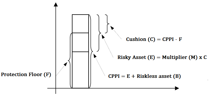
Run a Constant Proportion Portfolio Insurance (CPPI) strategy: 
- Keep exposure in a risky asset for upside potential, while ensuring capital preservation by increasing allocation to a safe asset if your portfolio value is nearing a set floor.
In [2]:
ind_return = erk.get_ind_returns()

# simulate returns from a safer asset, like bonds,
# using geometric brownian motion
safe_r = erk.gbm(
    n_years=10,
    n_scenarios=1,
    mu=0.03,
    sigma=0.015
).pct_change().dropna()

# retrieve telecom returns from 2005 to 2014
# some processing so it runs properly in run_cppi()
risky_r = ind_return.loc['2005':'2014', 'Telcm'].reset_index().drop('index', axis=1)
risky_r.columns = [0]

# CPPI with monthly rebalances
# m = cushion multiplier
backtest = erk.run_cppi(
    risky_r=risky_r,
    safe_r=safe_r,
    m=2,
    start=1000,
    floor=0.7,
)
Plot performance of CPPI strategy (black) vs strategy of allocating 100% of portfolio to the risky asset (orange)
- Set protection floor F to 70% of the initial investment
In [3]:
fig, ax = plt.subplots(figsize=(12,6))
backtest['Wealth'].plot(ax=ax, color='k', legend=False)
backtest['Risky Wealth'].plot(ax=ax, color='orange', style='--', legend=False)
ax.axhline(1000*0.8, color='red', linestyle='--')
plt.show()

Explore how adjusting CPPI parameters affects floor violations 
How does increasing the cusion multiplier m from 2 to 3 affect floor violations? Notice in the above example, there were no floor violations in the above case with m=2
In [4]:
# CPPI with monthly rebalances
# m = cushion multiplier
backtest = erk.run_cppi(
    risky_r=risky_r,
    safe_r=safe_r,
    m=3,
    start=1000,
    floor=0.7,
)
In [5]:
fig, ax = plt.subplots(figsize=(12,6))
backtest['Wealth'].plot(ax=ax, color='k', legend=False)
backtest['Risky Wealth'].plot(ax=ax, color='orange', style='--', legend=False)
ax.axhline(1000*0.8, color='red', linestyle='--')
plt.show()

With m=3, we had a floor violation during the '08 recession. Check what the portfolio value dropped to.
Remember our floor value was set to 80% of the initial 1000 investment = 800
In [6]:
backtest['Wealth'].min()
Out[6]:
Utilize a max drawdown constraint to create a moving floor. Set the floor value to 70% of max(peak, account_value)
In [7]:
# with m=3, floor value being 70% of max(peak, account_value),
# max allocation to risky assket is 3*(100-70) = 90%
backtest = erk.run_cppi(
    risky_r=risky_r,
    safe_r=safe_r,
    m=3,
    start=1000,
    riskfree_rate=0.02,
    drawdown=0.3
)
In [8]:
fig, ax = plt.subplots(figsize=(12,6))
backtest['Wealth'].plot(ax=ax, color='k', legend=False)
backtest['Risky Wealth'].plot(ax=ax, color='orange', style='--', legend=False)
ax.axhline(1000*0.8, color='red', linestyle='--')
plt.show()

Summary of CPPI's returns
In [9]:
erk.summary_stats(backtest['Wealth'].pct_change().dropna())
Out[9]:
Summary of 100% Telecom returns
In [10]:
erk.summary_stats(backtest['Risky Wealth'].pct_change().dropna())
Out[10]:
CPPI strategy provided much better risk protection
- Max drawdown was halved,
- Negative skewness reduced,
- VaR and CVar near halved
- Higher Sharpe ratio
- Much less fat tail on distribution of monthly returns (kurtosis)
Although, overall, it underperformed because of the run from 2009-2015